Global-Local Regularization Via Distributional Robustness
July 25, 2023
1. Introduction
As the Wasserstein (WS) distance is a powerful and convenient tool of measuring closeness between distributions, Wasserstein Distributional Robustness (WDR) has been one of the most widely-used variants of DR. Here we consider a generic Polish space endowed with a distribution . Let be a real-valued (risk) function and be a cost function. Distributional robustness setting aims to find the distribution in the vicinity of and maximizes the risk in the expectation form [1, 2]:
where and denotes an optimal transport (OT) or a WS distance with the set of couplings whose marginals are and .
Direct optimization over the set of distributions is often computationally intractable except in limited cases, we thus seek to cast this problem into its dual form. With the assumption that is upper semi-continuous and the cost is a non-negative and continuous function satisfying , [1, 2] showed the dual form is:
When applying DR to the supervised learning setting, is a pair of data/label drawn from and is the loss function [1, 2]. The fact that engages only certainly restricts the modeling capacity of the above equation. The reasons are as follows. Firstly, for each anchor , the most challenging sample is currently defined as the one maximizing , where is inherited from the primal form. Hence, it is not suitable to express the risk function engaging both and (e.g., Kullback-Leibler divergence between the predictions for and as in TRADES [3]). Secondly, it is also \emph{impossible} to inject a \emph{global regularization term} involving a batch of samples and .
Contribution. To empower the formulation of DR for efficiently tackling various real-world problems, in this work, we propose a rich OT-based DR framework, named Global-Local Regularization Via Distributional Robustness (GLOT-DR). Specifically, by designing special joint distributions and together with some constraints, our framework is applicable to a mixed variety of real-world applications, including domain generalization (DG), domain adaptation (DA), semi-supervised learning (SSL), and adversarial machine learning (AML).
Additionally, our GLOT-DR makes it possible for us to equip not only a for enforcing a local smoothness and robustness, but also a to impose a global effect targeting a downstream task. Moreover, by designing a specific WS distance, we successfully develop a closed-form solution for GLOT-DR without using the dual form.
Technically, our solution turns solving the inner maximization in the dual form into sampling a set of challenging particles according to a local distribution, on which we can handle efficiently using Stein Variational Gradient Decent (SVGD) [4] approximate inference algorithm. Based on the general framework of GLOT-DR, we establish the settings for DG, DA, SSL, and AML and conduct experiments to compare our GLOT-DR to state-of-the-art baselines in these real-world applications. Overall, our contributions can be summarized as follows:
We enrich the general framework of DR to make it possible for many real-world applications by enforcing both local and global regularization terms. We note that the global regularization term is crucial for many downstream tasks.
We propose a closed-form solution for our GLOT-DR without involving the dual form in [1, 2]. We note that the dual form is due to the minimization over .
We conduct comprehensive experiments to compare our GLOT-DR to state-of-the-art baselines in DG, DA, SSL, and AML. The experimental results demonstrate the merits of our proposed approach and empirically prove that both of the introduced local and global regularization terms advance existing methods across various scenarios, including DG, DA, SSL, and AML.
2. Proposed framework
We propose a regularization technique based on optimal transport distributional robustness that can be widely applied to many settings including i) , ii) , iii) , and iv) . In what follows, we present the general setting along with the notations used throughout the paper and technical details of our framework.
Figure 1: Overview of our proposed GLOT-DR framework
Assume that we have with the distributions and a with the distribution . For the -th source domain, we draw a batch of examples as , where . Meanwhile, for the target domain, we sample a batch of examples as .
It is worth noting that for the DG setting, we set (i.e., not use any target data in training). Furthermore, we examine the multi-class classification problem with the label set .
Hence, the prediction of a classifier is a prediction probability belonging to the m-1 . Finally, let with be parameters of our deep net, wherein is the feature extractor and is the classifier on top of feature representations.
Constructing Challenging Samples. As explained below, our method involves the construction of a random variable with distribution and another random variable with distribution , containing anchor samples and their perturbed counterparts .
The inclusion of both anchor samples and perturbed samples allows us to define a unifying cost function containing local regularization, global regularization, and classification loss.
Concretely, we first start with the construction of , containing repeated anchor samples as follows:
Here, each source sample is repeated times , while each target sample is repeated times . The corresponding distribution of this random variable is denoted as . In contrast to , we next define random variable , whose form is
Here we note that for , the index specifies the -th source domain, the index specifies an example in the -th source batch, while the index specifies the -th perturbed example to the source example . Similarly, for , the index specifies an example in the target batch, while the index specifies the -the perturbed example to the target example .
We would like to contain both: i) anchor examples, i.e., and ; ii) perturbed source samples to and perturbed target samples to . In order to impose this requirement, we only consider sampling from distribution inside the Wasserstein-ball of , i.e., satisfying
Here we slightly abuse the notion by using to represent its corresponding one-hot vector. By definition, this cost metric almost surely: i) enforces all -th (i.e., ) samples in to be anchor samples, i.e., ; ii) allows perturbations on the input data, i.e., and , for ; iii) restricts perturbations on labels, i.e., for (see Figure 1 for the illustration). The reason is that if either (i) or (iii) is violated on a non-zero measurable set then becomes infinity.
Learning Robust Classifier. Upon clear definitions of and , we wish to learn good representations and regularize the classifier , via the following DR problem:
The cost function with is defined as the weighted sum of a , a , and the , whose explicit forms are dependent on the task (DA, SSL, DG, and AML).
Intuitively, the optimization iteratively searches for the worst-case w.r.t. the cost , then changes the network to minimize the worst-case cost.
Training Procedure of Our Approach In what follows, we present how to solve the above optimization efficiently. Accordingly, we first need to sample . For each source anchor , we sample
in the ball with the to . Furthermore, for each target anchor , we sample in the ball with the to .
To sample the particles from their local distributions, we use Stein Variational Gradient Decent (SVGD) [4] with a RBF kernel with kernel width . Obtained particles and are then utilized to minimize the objective function for updating . Specifically, we utilize cross-entropy for the classification loss term and the symmetric Kullback-Leibler (KL) divergence for the local regularization term as
Finally, the global-regularization function of interest is defined accordingly depending on the task.
3. Experiments
To demonstrate the effectiveness of our proposed method, we evaluate its performance on various experiment protocols, including DG, DA, SSL, and AML. We tried to use the exact configuration of optimizers and hyper-parameters for all experiments and report the original results in prior work, if possible.
3.1 Experiments for domain generalization
Table 1: Single domain generalization accuracy (%) on CIFAR-10-C and CIFAR-100-C datasets with different backbone architectures. We use the bold font to highlight the best results.
Table 1 shows the average accuracy when we alternatively train the model on one category and evaluate on the rest. In every setting, GLOT-DR outperforms other methods by large margins. Specifically, our method exceeds the second-best method ME-ADA by on CIFAR-10-C and on CIFAR-100-C. The substantial gain in terms of the accuracy on various backbone architectures demonstrates the high applicability of our GLOT-DR.
Furthermore, we examine multi-source DG where the classifier needs to generalize from multiple source domains to an unseen target domain on the PACS dataset. Our proposed method is applicable in this scenario since it is designed to better learn domain invariant features as well as leverage the diversity from generated data. We compare GLOT-DR against DSN, L-CNN, MLDG, Fusion, MetaReg, Epi-FCR, AGG, HE, and PAR. Table 2 shows that our GLOT-DR outperforms the baselines for three cases and averagely surpasses the second-best baseline by . The most noticeable improvement is on the Sketch domain (, which is the most challenging due to the fact that the styles of the images are colorless and far different from the ones from Art Painting, Cartoon or Photos (i.e., larger domain shift).
Table 2: Multi-source domain generalization accuracy (%) on PACS datasets. Each column title indicates the target domain used for evaluation, while the rest are for training.
3.2 Experiments for domain adaptation
In this section, we conduct experiments on the commonly used dataset for real-world unsupervised DA – Office-31, comprising images from three domains: Amazon (A), Webcam (W) and DSLR (D). Our proposed GLOT-DR is compared against baselines: ResNet-50, DAN, RTN, DAN, JAN, GTA, CDAN, DeepJDOT and ETD . For a fair comparison, we follow the training setups of CDAN and compare with other works using this configuration. As can be seen from Table 2, GLOT-DR achieves the best overall performance among baselines with accuracy. Compared with ETD, which is another OT-based domain adaptation method, our performance significantly increases by on A W task, on W A and on average.
Table 3: Accuracy (%) on Office-31 (Saenko et al., 2010) of ResNet50 model (He et al., 2016) in unsupervised DA methods.
3.3 Experiments for semi-supervised learning
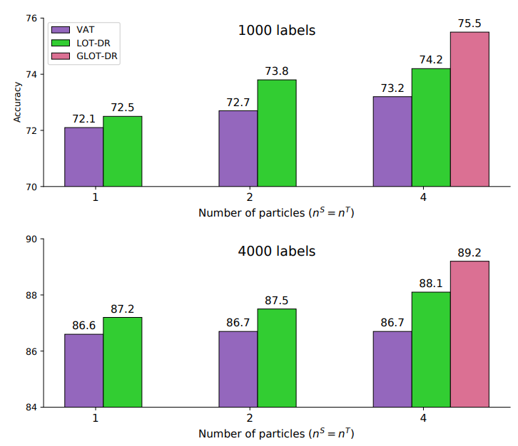
Sharing a similar objective with DA, which utilizes the unlabeled samples for improving the model performance, SSL methods can also benefit from our proposed technique. We present the empirical results on CIFAR-10 benchmark with ConvLarge architecture, following VAT’s protocol VAT, which serves as a strong baseline in this experiment. Results in Figure 3 (when training with 1,000 and 4,000 labeled examples) demonstrate that, with only perturbed sample per anchor, the performance of LOT-DR slightly outperforms VAT with . With more perturbed samples per anchor, this gap increases: approximately when and when . Similar to the previous DA experiment, adding the global regularization term helps increase accuracy by in this setup.
Figure 3: Accuracy (%) on CIFAR-10 of ConvLarge modelin SSL settings when using 1,000 and 4,000 labeled examples (i.e. 100 and 400 labeled samples each class). Best viewed in color
3.4 Experiments for adversarial machine learning
Table 4 shows the evaluation against adversarial examples. We compare our method with PGD-AT [6] and TRADES [3], two well-known defense methods in AML and SAT . For the sake of fair comparison, we use the same adversarial training setting for all methods, which is carefully investigated in [5]. We also compare with adversarial distributional training methods (ADT-EXP and ADT-EXPAM), which assume that the adversarial distribution explicitly follows normal distribution. It can be seen from Table 4 that our GLOT-DR method outperforms all these baselines in both natural and robustness performance. Specifically, compared to PGD-AT, our method has an improvement of 0.8 in natural accuracy and around 1 robust accuracies against PGD200 and AA attacks. Compared to TRADES, while achieving the same level of robustness, our method has a better performance with benign examples with a gap of 2.5. Especially, our method significantly outperforms ADT by around 7 under the PGD200 attack.
Table 4: Adversarial robustness evaluation on CIFAR10 of ResNet18 model. PGD, AA and B&B represent the robust accuracy against the PGD attack (with 10/200 iterations) (Madry et al., 2018), Auto-Attack (Croce and Hein, 2020) and B&B attack (Brendel et al., 2019), respectively, while NAT denotes the natural accuracy. Note that ⋆ results are taken from Pang et al. (Pang et al., 2020), while ⋄ results are our reproduced results.
3.4. Conclusion
Although DR is a promising framework to improve neural network robustness and generalization capability, its current formulation shows some limitations, circumventing its application to real-world problems. Firstly, its formulation is not sufficiently rich to express a global regularization effect targeting many applications. Secondly, the dual form is not readily trainable to incorporate into the training of deep learning models. In this work, we propose a rich OT based DR framework, named Global-Local Regularization Via Distributional Robustness (GLOT-DR) which is sufficiently rich for many real-world applications including DG, DA, SSL, and AML and has a closed-form solution. Finally, we conduct comprehensive experiments to compare our GLOT-DR with state-of-the-art baselines accordingly. Empirical results have demonstrated the merits of our GLOT-DR on standard benchmark datasets.
References
[1] Blanchet, J. and Murthy, K. (2019). Quantifying distributional model risk via optimal transport. Mathematics of Operations Research, 44(2):565–600.
[2] Sinha, A., Namkoong, H., and Duchi, J. (2018). Certifying some distributional robustness with principled adversarial training. In International Conference on Learning Representations.
[3] Zhang, H., Yu, Y., Jiao, J., Xing, E., El Ghaoui, L., and Jordan, M. (2019). Theoretically principled trade-off between robustness and accuracy. In Proceedings of ICML, pages 7472–7482. PMLR.
[4] Liu, Q. and Wang, D. (2016). Stein variational gradient descent: A general purpose bayesian inference algorithm. In Lee, D., Sugiyama, M., Luxburg, U., Guyon, I., and
Garnett, R., editors, Proceedings of NeurIPS, volume 29.
[5] Pang, T., Yang, X., Dong, Y., Su, H., and Zhu, J. (2020). Bag of tricks for adversarial training. In International Conference on Learning Representations.
[6] Madry, A., Makelov, A., Schmidt, L., Tsipras, D., and Vladu, A. (2018). Towards deep learning models resistant to adversarial attacks. In International Conference on Learning Representations.
 endowed with a distribution
  . Let
. Let  be a real-valued (risk) function and
  be a cost function. Distributional robustness setting aims to find the distribution
  in the vicinity of
 ![\[\sup_{\mathbb{\tilde{P}}:\mathcal{W}_{c}\left(\mathbb{P},\mathbb{\tilde{P}}\right)<\epsilon}\underset{\tilde{Z}\sim\mathbb{\mathbb{\tilde{P}}}}{\mathbb{E}}\left[r\left(\tilde{Z}\right)\right],\]](https://research.vinai.io/wp-content/ql-cache/quicklatex.com-0385d3d6d07faf283bcf407eaa147deb_l3.svg "Rendered by QuickLaTeX.com")
 and
and  denotes an optimal transport (OT) or a WS distance with the set of couplings
  whose marginals are
  .
. is upper semi-continuous and the cost
  is a non-negative and continuous function satisfying
  , [1, 2] showed the dual form is:
![\[\inf_{\lambda\geq0}\left\{ \lambda\epsilon+\mathbb{E}_{Z\sim\mathbb{P}}[\sup_{\tilde{Z}}\left\{ r\left(\tilde{Z}\right)-\lambda c\left(\tilde{Z},Z\right)\right\} ]\right\}.\]](https://research.vinai.io/wp-content/ql-cache/quicklatex.com-29b4e31d2117121079ccf7918dcadd6c_l3.svg "Rendered by QuickLaTeX.com")
 is a pair of data/label drawn from
  and
and  is the loss function [1, 2]. The fact that
  certainly restricts the modeling capacity of the above equation. The reasons are as follows. Firstly, for each anchor
  , the most challenging sample
  is currently defined as the one maximizing
  , where
  is inherited from the primal form. Hence, it is not suitable to express the risk function
  between the predictions for
  for enforcing a local smoothness and robustness, but also a
  to impose a global effect targeting a downstream task. Moreover, by designing a specific WS distance, we successfully develop a closed-form solution for GLOT-DR without using the dual form.
 due to the minimization over
  .
. , ii)
, ii)  , iii)
  , and iv)
  . In what follows, we present the general setting along with the notations used throughout the paper and technical details of our framework.
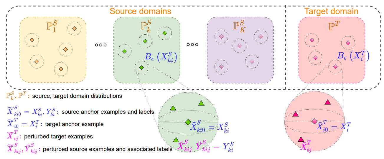
 with the
  distributions
  and a
and a  with the
  distribution
  . For the
  -th source domain, we draw a batch of
  examples as
  , where
  . Meanwhile, for the target domain, we sample a batch of
  examples as
  .
. (i.e., not use any target data in training). Furthermore, we examine the multi-class classification problem with the label set
  .
. . Finally, let
  with
with  be parameters of our deep net, wherein
  is the feature extractor and
  is the classifier on top of feature representations.
 and their perturbed counterparts
  .
.![\[Z :=\left[\left[\left[X_{kij}^{S},Y_{kij}^{S}\right]_{k=1}^{K}\right]_{i=1}^{B_{k}^{S}}\right]_{j=0}^{n^{S}},\left[\left[X_{ij}^{T}\right]_{i=1}^{B^{T}}\right]_{j=0}^{n^{T}}.\]](https://research.vinai.io/wp-content/ql-cache/quicklatex.com-543169572aff7b04a2dfddfd8bc09b48_l3.svg "Rendered by QuickLaTeX.com")
 times
times  , while each target sample is repeated
  times
times  . The corresponding distribution of this random variable is denoted as
  , whose form is
![\[\tilde{Z}:=\left[\left[\left[\tilde{X}_{kij}^{S},\tilde{Y}_{kij}^{S}\right]_{k=1}^{K}\right]_{i=1}^{B_{k}^{S}}\right]_{j=0}^{n^{S}},\left[\left[\tilde{X}_{ij}^{T}\right]_{i=1}^{B^{T}}\right]_{j=0}^{n^{T}}.\]](https://research.vinai.io/wp-content/ql-cache/quicklatex.com-19504f5cb1497513c0f54a90f9df5252_l3.svg "Rendered by QuickLaTeX.com")
 , the index
  specifies an example in the
  specifies the
  . Similarly, for
  , the index
  .
. and
and  ; ii)
; ii)  perturbed source samples
  to
to  and
and  perturbed target samples
  to
to ![\[\mathcal{W}_{\rho}\left(\mathbb{P},\tilde{\mathbb{P}}\right):=\underset{\gamma\in\Gamma\left(\mathbb{P},\tilde{\mathbb{P}}\right)}{\inf}\underset{\left(Z,\tilde{Z}\right)\sim\gamma}{\mathbb{E}}\left[\rho\left(Z,\tilde{Z}\right)\right]^{\frac{1}{q}}\leq\epsilon\]](https://research.vinai.io/wp-content/ql-cache/quicklatex.com-7559daa6a9fa80fbf6c5bb510edb84b0_l3.svg "Rendered by QuickLaTeX.com")
 to represent its corresponding one-hot vector. By definition, this cost metric almost surely: i) enforces all
  -th (i.e.,
  ) samples in
  ; ii) allows perturbations on the input data, i.e.,
  and
and  , for
, for  ; iii) restricts perturbations on labels, i.e.,
  for
for  (see Figure 1 for the illustration). The reason is that if either (i) or (iii) is violated on a non-zero measurable set then
  becomes infinity.
 , via the following DR problem:
![\[\min_{\theta,\phi}\max_{\tilde{\mathbb{P}}:\mathcal{W}_{\rho}\left(\mathbb{P},\tilde{\mathbb{P}}\right)\leq\epsilon}\mathbb{E}_{\tilde{Z}\sim\tilde{\mathbb{P}}}\left[r\left(\tilde{Z};\phi,\theta\right)\right].\]](https://research.vinai.io/wp-content/ql-cache/quicklatex.com-a1535450ba5d90e18dd1aca1d0e39568_l3.svg "Rendered by QuickLaTeX.com")
 with
with  is defined as the weighted sum of a
 , a
, a 
 , and the
 , whose explicit forms are dependent on the task (DA, SSL, DG, and AML).
 , then changes the network
  . For each source anchor
  , we sample
![\left[\tilde{X}_{kij}^{S}\right]_{j=1}^{n^{S}}\sim{q_{ki}^{S}}](https://research.vinai.io/wp-content/ql-cache/quicklatex.com-b140e1a93b2a525473f21c9fde38f089_l3.svg "Rendered by QuickLaTeX.com") in the ball
in the ball  with the
  to
to ![\exp\left\{ \lambda[\alpha s(X_{ki}^{S},\bullet;\psi)+\ell(\bullet,Y_{ki}^{S};\psi)]\right\}](https://research.vinai.io/wp-content/ql-cache/quicklatex.com-cac89464ba4f623555fd52fc5c8868c0_l3.svg "Rendered by QuickLaTeX.com") . Furthermore, for each target anchor
. Furthermore, for each target anchor  , we sample
 ![\left[\tilde{X}_{ij}^{T}\right]_{j=1}^{n^{T}}\sim{q_{i}^{T}}](https://research.vinai.io/wp-content/ql-cache/quicklatex.com-0f1ebf559a2ffab0a7497681fa90aaf2_l3.svg "Rendered by QuickLaTeX.com") in the ball
in the ball  with the
 .
. . Obtained particles
  and
and  are then utilized to minimize the objective function for updating
  and the symmetric Kullback-Leibler (KL) divergence for the local regularization term
  as
as 
![r^{g}\left(\left[X_{ki}^{S}\right]_{k,i},\left[X_{i}^{T}\right]_{i};\psi\right)](https://research.vinai.io/wp-content/ql-cache/quicklatex.com-d148a02bd094ef2686feda62452680f5_l3.svg "Rendered by QuickLaTeX.com") is defined accordingly depending on the task.
is defined accordingly depending on the task.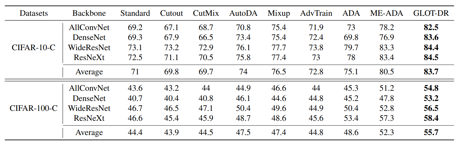
 on CIFAR-10-C and
  on CIFAR-100-C. The substantial gain in terms of the accuracy on various backbone architectures demonstrates the high applicability of our GLOT-DR.
 . The most noticeable improvement is on the Sketch domain (
 , which is the most challenging due to the fact that the styles of the images are colorless and far different from the ones from Art Painting, Cartoon or Photos (i.e., larger domain shift).
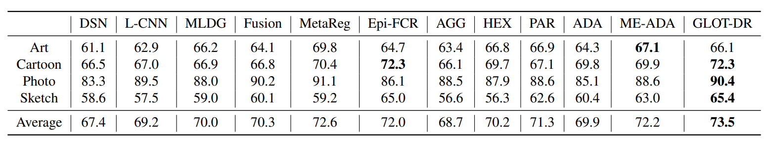
 accuracy. Compared with ETD, which is another OT-based domain adaptation method, our performance significantly increases by
  on A
on A W task,
  on W
on W on average.
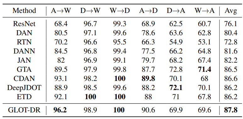
 perturbed sample per anchor, the performance of LOT-DR slightly outperforms VAT with
  . With more perturbed samples per anchor, this gap increases: approximately
  when
when  and
and  when
when  . Similar to the previous DA experiment, adding the global regularization term helps increase accuracy by
  in this setup.
 in natural accuracy and around 1