Denoising Probabilistic Models (DPMs) represent an emerging domain of generative models that excel in generating diverse and high-quality images. However, most current training methods for DPMs often neglect the correlation between timesteps, limiting the model’s performance in generating images effectively. Notably, we theoretically point out that this issue can be caused by the cumulative estimation gap between the predicted and the actual trajectory. To minimize that gap, we propose a novel Sequence-Aware (SA) loss to reduce the estimation gap to enhance the sampling quality. Furthermore, we theoretically show that our proposed loss function is a tighter upper bound of the estimation loss in comparison with the conventional loss in DPMs. Experimental results on several benchmark datasets including CIFAR10, CelebA, and CelebA-HQ consistently show a remarkable improvement of our proposed method regarding the image generalization quality measured by FID and Inception Score compared to several DPM baselines. Our code and pre-trained checkpoints are available at https://github.com/VinAIResearch/SA-DPM.
2. Background
Diffusion Probabilistic Models are comprised of two fundamental components, including the forward process and the reverse process. The former gradually diffuses each input , following a data distribution , into a standard Gaussian noise through timesteps, i.e., . The reverse process starts from and then iteratively denoises to get an original image. We recap the background of DPMs following the idea of DDPM [1].
2.1. Forward Process
Given an original data distribution , the forward process can be presented as follows:
where and an increasing noise scheduling sequence , which describes the amount of noise added at each timestep . Denoting and , the distribution of diffused image at timestep has a closed form as:
2.2. Reverse Process
The reverse conditional distribution can be approximated by a Gaussian conditional distribution
where and .
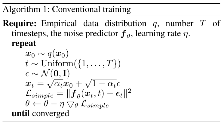
Instead of using the mean predicted by the denoising model, one can use a noise prediction model that predicts the noise added to to construct . This allows training by simply minimizing the mean squared error between the predicted noise and the true added Gaussian noise (detailed in Algorithm 1):
3. Method
In the sampling phase, a small amount of error may be introduced in each denoising iteration due to the imperfect learning process. Note that the inference process often requires many iterations to produce high-quality images, leading to the accumulation of these errors. In this section, we first point out the estimation gap between the predicted and ground-truth noises in the sampling process of DPMs and show its importance in the training phase to mitigate this accumulation and improve the quality of generated images. Based on that gap, we introduce a novel loss function that is proven to be tighter than commonly used in DPMs.
3.1. Estimation Gap
Figure 1: 1-D example of sampling trajectory. Under the assumption that the error at each timestep is similar: (a) the cumulative error by steps is large while (b) the cumulative error by steps is small. This behaviour is due to the correlation between neighbour timesteps.
Theorem 1 (Estimation gap):
Let be a noise predictor with parameter . Its total gap from step 2 to , for each , is
where . Furthermore, the total loss of is .
In typical DPMs, the training process is often performed by minimizing the conventional square loss at each step , which may not necessarily minimize . It means that minimizing can produce multiple small gaps . In the worst case, it ignores the relationship between timesteps, which may cause a large total gap at the end of the trajectory as visualized by a 1-D example in Figure 1a.
Therefore, a better way to train a DPM is to directly minimize the total gap , instead of trying to minimize each independent term . That scenario can be intuitively illustrated in Figure 1b.
3.2. Sequence-aware Training
Minimizing directly the whole is challenging due to the requirement of a large number of timesteps, which often leads to a significant memory and computation capability in the training phase. To address that issue, we propose to minimize the local gap that connects consecutive steps (for ).
The sequence-aware (SA) loss function for training is:
where and for any .
However, we found that optimizing that function independently makes the training error at each timestep quite large, since this SA loss does not strongly constrain the error at individual steps. Therefore, we suggest optimizing jointly with to exploit their advantages, resulting in the following total loss function for training DPMs:
where is a hyper-parameter that indicates how much we constrain the sampling trajectory. Optimizing the new loss term involves the direction of error at each step. Algorithm 2 represents the training procedure.
3.3. Bounding the Estimation Gap
We have presented the new loss which incorporates more information of the sequential nature of DPMs. We next theoretically show that this loss is tighter than the vanilla loss.
Theorem 2:
Let be any noise predictor with parameter . Consider the weighted conventional loss function , where is defined in Theorem 1 and . Then
4. Experiments
4.1. Image Generation
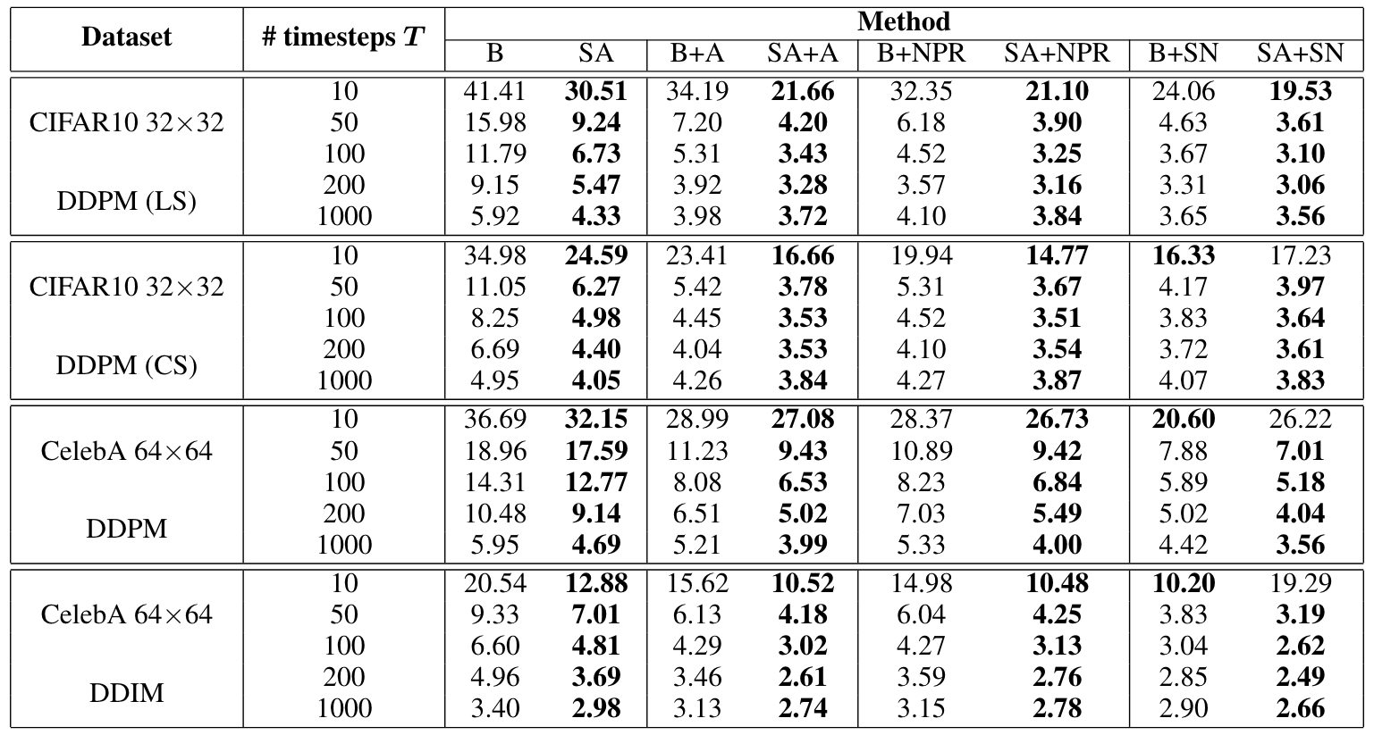
Table 1: FID score (). The results are reported under different numbers of timesteps . Here B and SA denote the baseline and our proposed method. A, NPR, and SN denote Analytic-DPM, NPR-DPM, and SN-DPM, respectively.
Table 2: IS metric ().
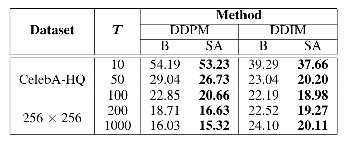
Table 3: FID score (). The results are reported under different number of timesteps. Here B and SA denote the baseline and our proposed loss.
Figure 3: Qualitative results of CelebA-HQ 256 256.
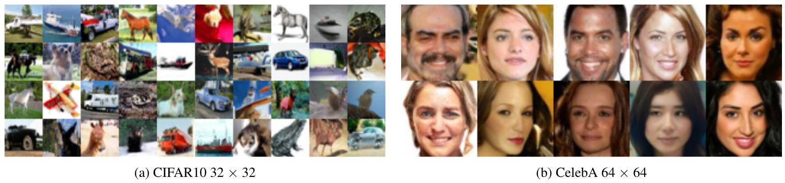
Tables 1, 2, and 3 demonstrate the substantial improvement of SA-2-DPM over the original DPM [1,4] especially when the number of timesteps decreases across datasets like CIFAR10, CelebA, and CelebA-HQ. As observed from those tables, for many settings, 50 or 100 timesteps are sufficient for our method to achieve a similar FID level with prior methods that use 1000 timesteps. For qualitative results, we provide the generated samples of our SA-2-DPM in Figures 2 and 3.
In addition, we also combine our proposed loss with the three covariance estimation methods (Analytic-DPM [2], NPR-DPM, and SN-DPM [3]) on two datasets: CIFAR10 and CelebA. Tables 1 and 2 show that our loss can significantly boost the image quality. This could be attributed to the capability of our loss to enhance the estimation of the mean of the backward Gaussian distributions in the sampling procedure. So when incorporating the additional covariance estimation methods, the generated image quality is further improved.
4.2. Ablation Study on the Weight
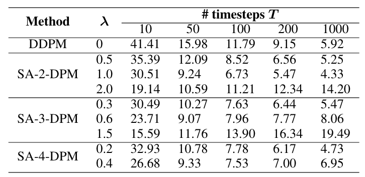
Table 4: FID of CIFAR10 dataset under different weight of . We use the sampling type of DDPM to synthesize.
In this part, we consider the variations in FID scores for the CIFAR10 dataset across different configurations of weight . As presented in Table 4, all the tested SA--DPM methods yield better results compared to the vanilla DPM. With different numbers of consecutive steps, the weight plays a crucial role. Specifically, SA-2-DPM (), SA-3-DPM (), and SA-4-DPM () consistently outperform DPM for all numbers of sampling timesteps. However, when the weight is set much higher, the quality of generated images will degrade slightly when using a large number of timesteps (e.g., 1000), even though it will be significantly better when using a small number of timesteps.
4.3. Evaluation on the Estimation Gap
Figure 4: Total gap term when sampling image starting from on CIFAR10 dataset.
In this experiment, we evaluate the total gap term of each trained model during sampling. Figure 4 illustrates of the sampling process of four trained models on the CIFAR10 dataset. It can be observed that when training with more consecutive timesteps in , the total gap term is more effectively minimized during the sampling process. Specifically, with SA-2-DPM, at the final timestep of the denoising process, the total gap term is reduced by approximately 2.5 times compared to the base model.
5. Conclusion
In this work, we examine the estimation gap between the ground truth and predicted trajectory in the sampling process of DPMs. We then propose a sequence-aware loss, that optimizes multiple timesteps jointly to leverage their sequential relationship. We theoretically prove that our proposed loss is a tighter upper bound of the estimation gap than the vanilla loss. Our experimental results verify that our loss reduces the estimation gap and enhances the sample quality. Moreover, when combining our loss with advanced techniques, we achieve a significant improvement over the baselines. Therefore, with our new loss, we provide a new benchmark for future research on DPMs. This new loss represents the true loss of a sampling step and therefore may facilitate future deeper understandings of DPMs, such as generalization ability and optimality. One limitation of this work is that our new loss requires the calculation of the network’s output at many timesteps, which makes the training time longer compared to the vanilla loss.
Key References
[1] Jonathan Ho, Ajay Jain, and Pieter Abbeel. Denoising diffusion probabilistic models. Advances in neural information processing systems, 33:6840–6851, 2020.
[2] Fan Bao, Chongxuan Li, Jun Zhu, and Bo Zhang. Analytic-DPM: an analytic estimate of the optimal reverse variance in diffusion probabilistic models. In International Conference on Learning Representations, 2022.
[3] Fan Bao, Chongxuan Li, Jiacheng Sun, Jun Zhu, and Bo Zhang. Estimating the optimal covariance with imperfect mean in diffusion probabilistic models. In International Conference on Machine Learning, pages 1555–1584. PMLR, 413 2022.
[4] Jiaming Song, Chenlin Meng, and Stefano Ermon. Denoising diffusion implicit models. In International Conference on Learning Representations, 2021.
 , following a data distribution
  , into a standard Gaussian noise through
  timesteps, i.e.,
  . The reverse process starts from
  and then iteratively denoises to get an original image. We recap the background of DPMs following the idea of DDPM [1].
![\[q(\boldsymbol{x}_{1:T}|\boldsymbol{x}_{0}) = \prod_{t=1}^{T} q(\boldsymbol{x}_{t}|\boldsymbol{x}_{t-1}),\]](https://research.vinai.io/wp-content/ql-cache/quicklatex.com-5dddf07ea043b839e14ed8ad34c7c6f7_l3.svg "Rendered by QuickLaTeX.com")
 and an increasing noise scheduling sequence
 ![\beta_{t} \in (0, 1]](https://research.vinai.io/wp-content/ql-cache/quicklatex.com-f7557f07bcd278619c5e44b43826ae8c_l3.svg "Rendered by QuickLaTeX.com") , which describes the amount of noise added at each timestep
, which describes the amount of noise added at each timestep  . Denoting
  and
and  , the distribution of diffused image
  at timestep
 ![\[q(\boldsymbol{x}_{t}|\boldsymbol{x}_{0}) = \mathcal{N}(\boldsymbol{x}_{t}; \sqrt{\bar{\alpha}_{t}}\boldsymbol{x}_{0}, (1-\bar{\alpha}_{t})\mathbf{I}).\]](https://research.vinai.io/wp-content/ql-cache/quicklatex.com-b34f53cf838ce2c9469354b72f269f59_l3.svg "Rendered by QuickLaTeX.com")
 can be approximated by a Gaussian conditional distribution
 ![\[q(\boldsymbol{x}_{t-1}|\boldsymbol{x}_{t},\boldsymbol{x}_0)=\mathcal{N}(\boldsymbol{x}_{t-1}; \tilde{\boldsymbol{\mu}}_{t}(\boldsymbol{x}_{t}, \boldsymbol{x}_{0}), \tilde{\beta}_{t}\mathbf{I}),\]](https://research.vinai.io/wp-content/ql-cache/quicklatex.com-1430e6619f75f5f9da39af98c2a58006_l3.svg "Rendered by QuickLaTeX.com")


 and
and  .
. predicted by the denoising model, one can use a noise prediction model
  that predicts the noise
  added to
  and the true added Gaussian noise
 ![\[\mathcal{L}_{simple} &= \mathbf{E}_{t, \boldsymbol{x}_{0}, \epsilon_{t}}\mathlarger{[}\|\boldsymbol{f}_{\theta}(\boldsymbol{x}_{t},t) - \boldsymbol{\epsilon}_{t}\|^{2}\mathlarger{]}\]](https://research.vinai.io/wp-content/ql-cache/quicklatex.com-cae24da8bcc3e562476cd0d295ee2c71_l3.svg "Rendered by QuickLaTeX.com")
 commonly used in DPMs.
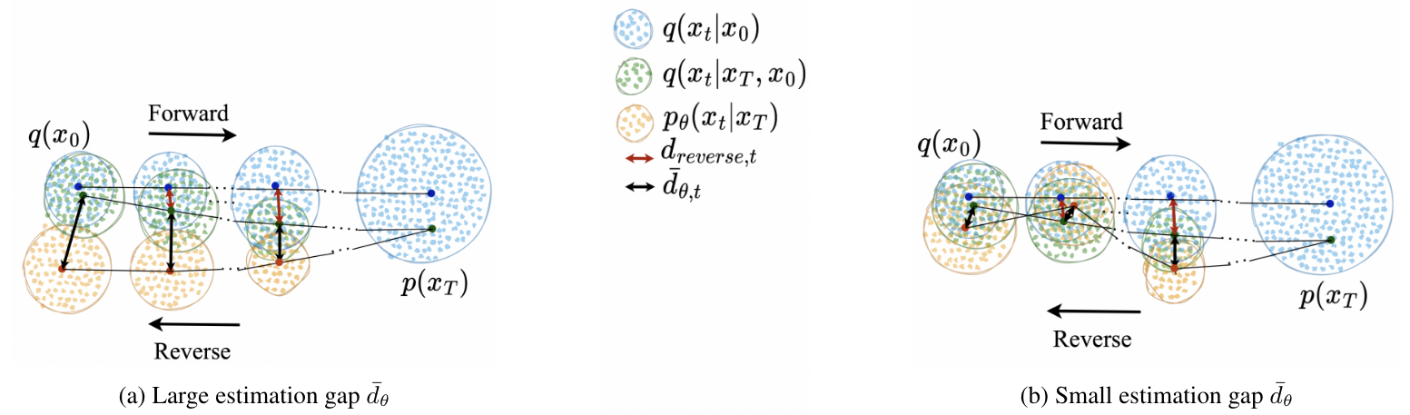
 be a noise predictor with parameter
  . Its total gap from step 2 to
  , is
, is ![\[d_{\theta}(\boldsymbol{x}_{0}) = \sum_{i=2}^{T}\tau_{i}(\boldsymbol{f}_{\theta}(\boldsymbol{x}_{i}, i) - \boldsymbol{\epsilon}_{i}),\]](https://research.vinai.io/wp-content/ql-cache/quicklatex.com-56e6c1fbf6447ff7eab0577eff521bdb_l3.svg "Rendered by QuickLaTeX.com")
 . Furthermore, the total loss of
  .
. at each step
  . It means that minimizing
  can produce multiple small gaps
  . In the worst case, it ignores the relationship between timesteps, which may cause a large total gap
  at the end of the trajectory as visualized by a 1-D example in Figure 1a.
 . That scenario can be intuitively illustrated in Figure 1b.
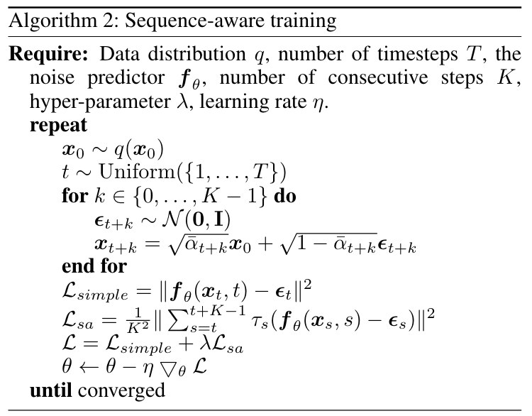
 consecutive steps (for
  ).
). ![\[\mathcal{L}_{sa} = \mathbf{E}_{t, \boldsymbol{x}_{0}, \boldsymbol{\epsilon}_{t: t+K-1}} \left\| \frac{1}{K} \sum_{s=t}^{t+K-1} \tau_{s}(\boldsymbol{f}_{\theta}(\boldsymbol{x}_{s}, s) - \boldsymbol{\epsilon}_{s}) \right\|^{2},\]](https://research.vinai.io/wp-content/ql-cache/quicklatex.com-5729ef9366563bdbf36cf503a3308a64_l3.svg "Rendered by QuickLaTeX.com")
 and
and  for any
  .
. jointly with
 ![\[\mathcal{L} = \mathcal{L}_{simple} + \lambda \mathcal{L}_{sa},\]](https://research.vinai.io/wp-content/ql-cache/quicklatex.com-b5fe88b0c55b030f17519074310d98b5_l3.svg "Rendered by QuickLaTeX.com")
 is a hyper-parameter that indicates how much we constrain the sampling trajectory. Optimizing the new loss term involves the direction of error at each step. Algorithm 2 represents the training procedure.
![\mathcal{L}_{simple}^{\tau} := \mathbf{E}_{t, \boldsymbol{x}_{0}, \boldsymbol{\epsilon}_{t}} \left[ \tau_{t}^2 \|\boldsymbol{f}_{\theta}(\boldsymbol{x}_{t}, t) - \boldsymbol{\epsilon}_{t}\|^{2}\right]](https://research.vinai.io/wp-content/ql-cache/quicklatex.com-ffa80f446ad28f98c0dd7405bf855c05_l3.svg "Rendered by QuickLaTeX.com") , where
, where  is defined in Theorem 1 and
  . Then
 ![\[\frac{T-1}{T+K} \mathcal{L}_{simple}^{\tau} \ge \mathcal{L}_{sa} \ge \frac{1}{(T+K)^2} \mathcal{L}_{\theta}.\]](https://research.vinai.io/wp-content/ql-cache/quicklatex.com-243d8ea67c52fe02a5b7a2185389b5a1_l3.svg "Rendered by QuickLaTeX.com")
 ). The results are reported under different numbers of timesteps
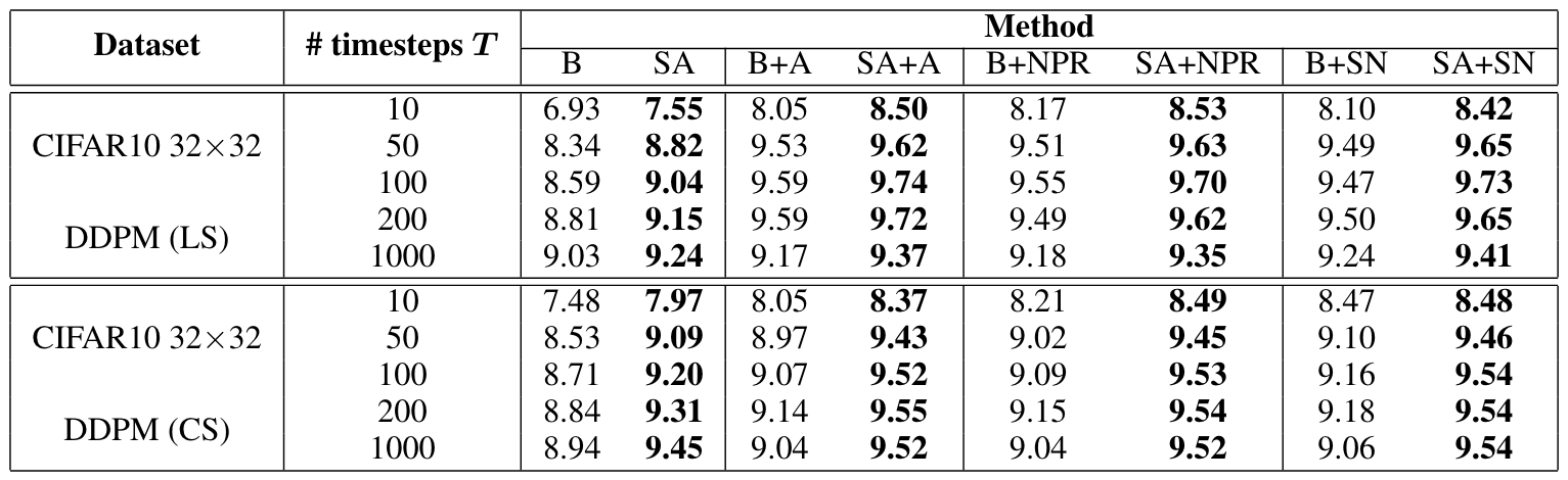
 ).
).
 32. (b) CelebA 64
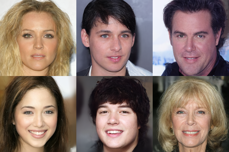

 ), SA-3-DPM (
 ), and SA-4-DPM (
 ) consistently outperform DPM for all numbers of sampling timesteps. However, when the weight
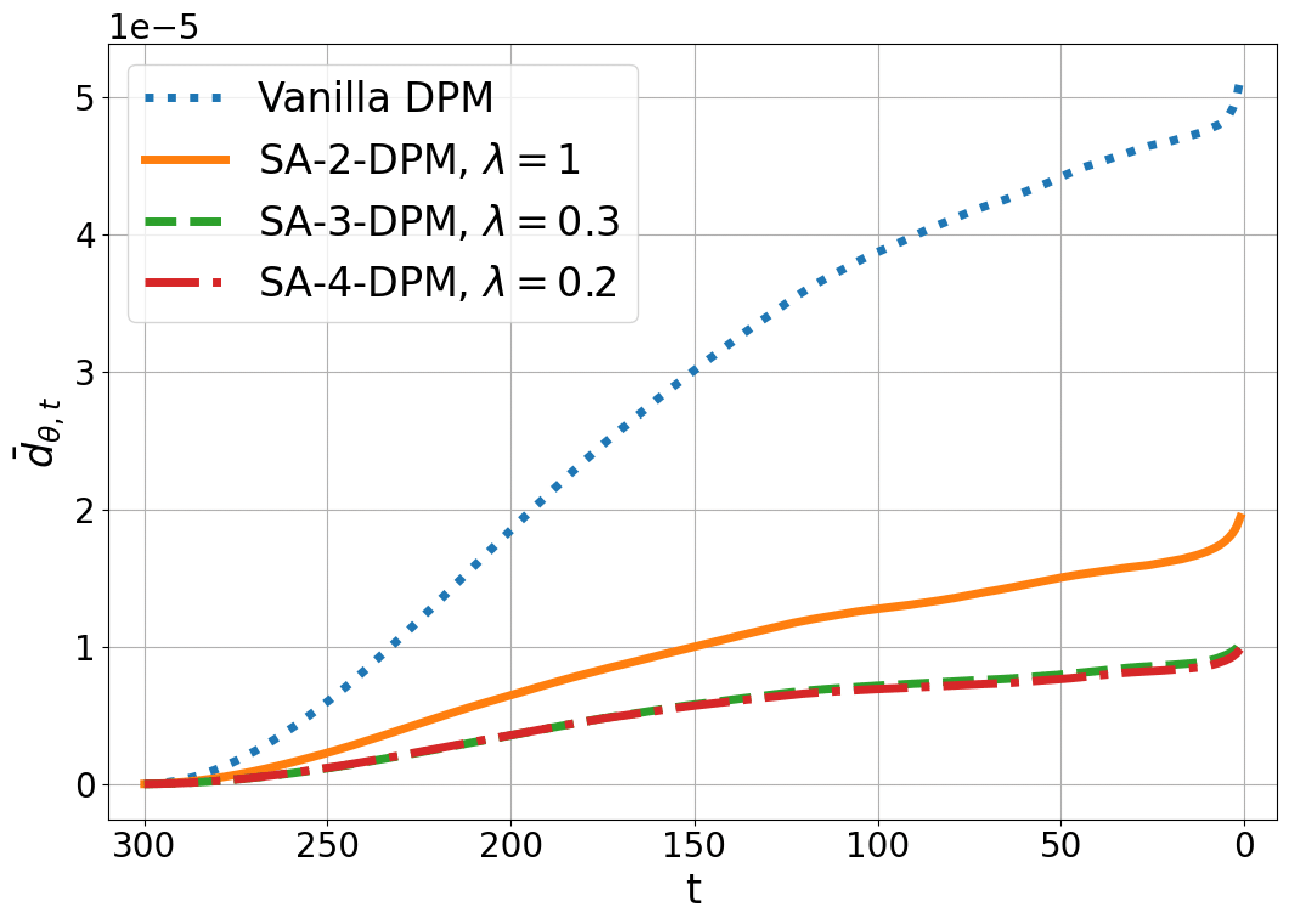
 when sampling image starting from
  on CIFAR10 dataset.